A function to calculate the slope and intercept of an amplification curve data from a quantitative PCR experiment at the end of the data stream.

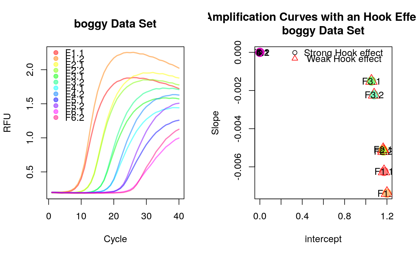
hookreg is a function to calculate the slope and intercept of an amplification curve data from a quantitative PCR experiment. The idea is that a strong negative slope at the end of an amplification curve is indicative for a hook effect (see Barratt and Mackay 2002).

hookreg(x, y, normalize = TRUE, sig.level = 0.0025,
  CI.level = 0.9975, robust = FALSE)

Arguments

x	is the cycle numbers (x-axis).
y	is the cycle dependent fluorescence amplitude (y-axis).
normalize	is a logical parameter indicating if the data should be normalized to the 0.999 quantile
sig.level	defines the significance level to test for a significant regression
CI.level	confidence level required for the slope
robust	is a logical parameter indicating if the data should be analyzed be a robust linear regression (lmrob).

References

K. Barratt, J.F. Mackay, Improving Real-Time PCR Genotyping Assays by Asymmetric Amplification, J. Clin. Microbiol. 40 (2002) 1571--1572. doi:10.1128/JCM.40.4.1571-1572.2002.

Examples

# Calculate slope and intercept on noise (negative) amplification curve data
# for the last eight cycles.

library(qpcR)

res_hook <- data.frame(sample=colnames(boggy)[-1],
                       t(sapply(2:ncol(boggy), function(i) {
                       hookreg(x=boggy[, 1], y=boggy[, i])})))
res_hook
#>    sample intercept        slope hook.start hook.delta      p.value
#> 1    F1.1  1.172270 -0.006245585         26         15 5.036934e-11
#> 2    F1.2  1.200001 -0.007383676         26         15 1.002592e-12
#> 3    F2.1  1.164265 -0.005088431         32          9 3.832008e-06
#> 4    F2.2  1.167357 -0.005181812         32          9 7.647282e-07
#> 5    F3.1  1.053409 -0.001504617         35          6 5.438867e-02
#> 6    F3.2  1.078725 -0.002225900         35          6 2.157723e-02
#> 7    F4.1  0.000000  0.000000000          0          0           NA
#> 8    F4.2  0.000000  0.000000000          0          0           NA
#> 9    F5.1  0.000000  0.000000000          0          0           NA
#> 10   F5.2  0.000000  0.000000000          0          0           NA
#> 11   F6.1  0.000000  0.000000000          0          0           NA
#> 12   F6.2  0.000000  0.000000000          0          0           NA
#>          CI.low        CI.up hook.fit hook.CI hook
#> 1  -0.007438201 -0.005052969        1       1    1
#> 2  -0.008419439 -0.006347914        1       1    1
#> 3  -0.006895532 -0.003281330        1       1    1
#> 4  -0.006633731 -0.003729894        1       1    1
#> 5  -0.005278075  0.002268842        0       0    0
#> 6  -0.006335882  0.001884081        0       0    0
#> 7            NA           NA        0       0    0
#> 8            NA           NA        0       0    0
#> 9            NA           NA        0       0    0
#> 10           NA           NA        0       0    0
#> 11           NA           NA        0       0    0
#> 12           NA           NA        0       0    0

data_colors <- rainbow(ncol(boggy[, -1]), alpha=0.5)
cl <- kmeans(na.omit(res_hook[, 2:3]), 2)$cluster

par(mfrow=c(1,2))
matplot(x=boggy[, 1], y=boggy[, -1], xlab="Cycle", ylab="RFU",
 main="boggy Data Set", type="l", lty=1, lwd=2, col=data_colors)
 legend("topleft", as.character(res_hook$sample), pch=19,
         col=data_colors, bty="n")

plot(res_hook$intercept, res_hook$slope, pch=19, cex=2, col=data_colors,
 xlab="intercept", ylab="Slope",
 main="Clusters of Amplification Curves with an Hook Effect-like Curvature\nboggy Data Set")
 points(res_hook$intercept, res_hook$slope, col=cl, pch=cl, cex=cl)
 legend("topright", c("Strong Hook effect", " Weak Hook effect"), pch=c(1,2), col=c(1,2), bty="n")
 text(res_hook$intercept, res_hook$slope, res_hook$sample)