Algorithms for Automatized Detection of Hook Effect-bearing Amplification Curves
The PCRedux package authors
2019-10-28
SI1.RmdThe PDF version of this document is available online.
The document is part of the publication M. Burdukiewicz, A.-N. Spiess, K.A. Blagodatskikh, W. Lehmann, P. Schierack, S. Rödiger, Algorithms for automated detection of hook effect-bearing amplification curves, Biomolecular Detection and Quantification. (2018). doi:10.1016/j.bdq.2018.08.001.
Abstract
This is a supplemental document for the study Algorithms for Automatized Detection of Hook Effect-bearing Amplification Curves. Quantitative real-time PCR (qPCR) is a widely used method for gene expression analysis, forensics and medical diagnostics (Dvinge and Bertone 2009; Martins et al. 2015; Sauer, Reinke, and Courts 2016).
Numerous algorithms have been developed to extract features from amplification curves such as the cycle of quantification and the amplification efficiency (Ruijter et al. 2013). There is an agreement, that these algorithms need to be evaluated and benchmarked for their performance (Kemperman and McCall 2017). But at an earlier level it is important to have a solid foundation for the data preprocessing (Spiess et al. 2015, 2016; Ronde et al. 2017). Digitalization of processes holds the promise that potential human mistakes can be spotted and that diagnostic processes can be automatized.
The aim of the study is to provide software tools and algorithms, which assists qPCR users during the analysis and quality management of their data. In particular, this study shows how it is possible to automatically detect hook effects (see Barratt and Mackay (2002)) or hook effect-like curvatures.
Introduction
The functions and data presented in the paper are available from https://github.com/devSJR/PCRedux. The data, including the RDML file, are part of the package and are made available in the CSV or RDML format (Rödiger et al. 2017) for vendors independent analysis.
All analyses were implemented and conducted with the R statistical computing language (R Core Team 2017; Rödiger et al. 2015) and dedicated integrated development environments such as RKWard (Rödiger et al. 2012). Further documentation can be found in the help files of the R packages.
Installation
The hookreg() and hookregNL() functions are part of the package for the R statistical computing language. Download from CRAN http://cran.r-project.org/ the R version for the required operating system and install R. Then start R and type in the prompt:
The package should just install. If this fails make sure you have write access to the destination directory and follow the instructions of the R documentation:
# The following command points to the help for download and install of packages
# from CRAN-like repositories or from local files.
?install.packages()
The package can be installed as the latest development version using the devtools R package.
# Install devtools, if you haven't already.
install.packages("devtools")

library(devtools)
install_github("devSJR/PCRedux")
It is recommended to use software with an integrated development environment such as (Rödiger et al. 2012). To work with RDML data it is recommend to use the package (\(\geq\)v.0.9-9) by invoking the rdmlEdit() function (for details see Rödiger et al. (2017)) or the rdmlEdit GUI web server (section ). The RDML file hookreg.rdml contains the amplification curve data. However, other software package (e.g., (Lefever et al. 2009; Ruijter et al. 2015)) can also be used to work with the RMDL data file format.
Results for the analysis of the hookreg.rdml data set by humanrater()
All calculations in the following sections were employed on the hookreg.rdml data R environment by the package (Rödiger et al. 2017). An overview of the used samples and the qPCR detection chemistries and the classification by two humans (“Hook effect-like Rater 1”, “Hook effect-like Rater 2”) is shown in Table .
Loading experiment: exp1 run: run1
All amplification curves were plotted according to their experiment conditions. They differed in the target molecules (e.g., , ) and the detection chemistries (e.g., EvaGreen, SybrGreen, hydrolysis probes). Figure shows seven plots for the corresponding experiments. The amplification curves were not preprocessed to preserve the curvature. Selected amplification curves were noisy (e.g., Figure F), had overshots or undershot in the background phase (e.g., Figure E-G), a short hook phase (e.g., Figure D). Amplification curves of Figure A, D, F and F exhibited a clearly visible hook effect or a hook like effect.
par(mfrow=c(4,2))

# Plot all data of the hookreg.rdml-file according to their type.
# Synthetic template, detected with Syto-13
matplot(data[, 1], data[, 2:13], type="l", lty=1, lwd=2, ylab="RFU", xlab="Cycle")
mtext("A", cex = 1.8, side = 3, adj = 0, font = 2)

# Human MLC-2v, detected with a hydrolysis probe.
matplot(data[, 1], data[, 14:45], type="l", lty=1, lwd=2, ylab="RFU", xlab="Cycle")
mtext("B", cex = 1.8, side = 3, adj = 0, font = 2)

# S27a housekeeping gene, detected with SybrGreen I.
matplot(data[, 1], data[, 46:69], type="l", lty=1, lwd=2, ylab="RFU", xlab="Cycle")
mtext("C", cex = 1.8, side = 3, adj = 0, font = 2)

# Whole genome amplification, detected with EvaGreen.
matplot(data[, 1], data[, 70:71], type="l", lty=1, lwd=2, ylab="RFU", xlab="Cycle")
mtext("D", cex = 1.8, side = 3, adj = 0, font = 2)

# Human BRCA1 gene, detected with a hydrolysis probe.
matplot(data[, 1], data[, 72:87], type="l", lty=1, lwd=2, ylab="RFU", xlab="Cycle")
mtext("E", cex = 1.8, side = 3, adj = 0, font = 2)

# Human NRAS gene, detected with a hydrolysis probe.
matplot(data[, 1], data[, 88:95], type="l", lty=1, lwd=2, ylab="RFU", xlab="Cycle")
mtext("F", cex = 1.8, side = 3, adj = 0, font = 2)

# Water control, detected with a hydrolysis probe.
matplot(data[, 1], data[, 96:97], type="l", lty=1, lwd=2, ylab="RFU", xlab="Cycle")
mtext("G", cex = 1.8, side = 3, adj = 0, font = 2)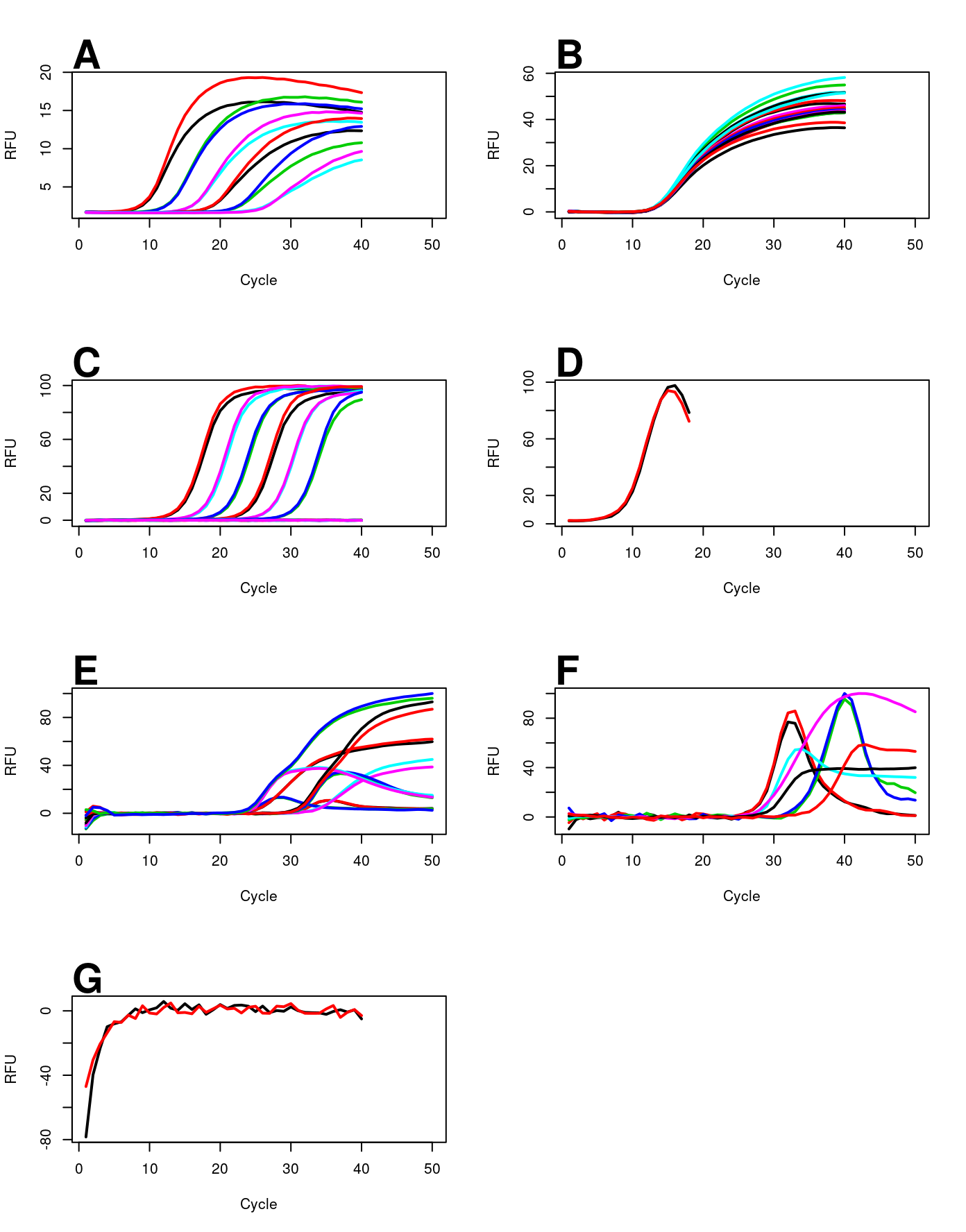
Amplification curves. A) Synthetic template, detected with Syto-13. B) Human , detected with a hydrolysis probe. C) housekeeping gene, detected with SybrGreen I. D) Whole genome amplification, detected with EvaGreen. E) Human gene, detected with a hydrolysis probe. F) Human gene, detected with a hydrolysis probe. G) Water control, detected with a hydrolysis probe. See Table for details. RFU, relative fluorescence units.
Printout of all measured samples, their rating by two humans (rater 1 and rater 2) with their dichotomous ratings (0, no hook; 1, hook) and their sources.
- The boggy data (qpcR::boggy) set was taken from the package (Ritz and Spiess 2008; Spiess, Feig, and Ritz 2008).
- The C127EGHP data (chipPCR::C127EGHP) set was taken from the package (Rödiger, Burdukiewicz, and Schierack 2015).
- The testdat data (qpcR::testdat) set was taken from the package (Ritz and Spiess 2008; Spiess, Feig, and Ritz 2008).
- Other data were prepared by Evrogen laboratory experiments.
Results for the analysis with hookreg() and hookregNL()
This section contains the results of the analysis of the amplification curve data with the hookreg() function and the hookregNL() function. As in the previous sections, all code was commented to make it reproducible. Some rows in Table and Table appear to be empty. This expected behavior may occur in cases where the corresponding functions were not able to calculate the coefficients due to a failed model fit or violation of the truncation criterion.
Results for the analysis of the hookreg.rdml data set with hookreg()
The following code was used to analyze the hookreg.rdml data set with hookreg() function. The hookreg() function fits a linear model to a region of interest. The linear model is used to decide if the amplification curve as a hook effect or hook effect-like curvature.
# Load PCRedux package to obtain the data and make the hookreg() function
# available.
library(PCRedux)

# `data` is a temporary data frame of the hook.rdml amplification curve data file.
# Apply the hookreg() function over the amplification curves and arrange the
# results in the data frame `res_hookreg`.

res_hookreg <-  data.frame(sample=colnames(data)[-1],
                           t(sapply(2L:ncol(data), function(i) {
                             hookreg(x=data[, 1], y=data[, i])
                           })))

# Fetch the calculated parameters from the calculations with the hookreg()
# function as a table `res_hookreg_table`.

res_hookreg_table <- data.frame(sample=as.character(res_hookreg[["sample"]]),
                                intercept=signif(res_hookreg[["intercept"]], 2),
                                slope=signif(res_hookreg[["slope"]], 1),
                                hook.start=signif(res_hookreg[["hook.start"]], 0),
                                hook.delta=signif(res_hookreg[["hook.delta"]], 0),
                                p.value=signif(res_hookreg[["p.value"]], 4),
                                CI.low=signif(res_hookreg[["CI.low"]], 2),
                                CI.up=signif(res_hookreg[["CI.up"]], 2),
                                hook.fit=res_hookreg[["hook.fit"]],
                                hook.CI=res_hookreg[["hook.CI"]],
                                hook=res_hookreg[["hook"]]
)
Finally a pretty printout (Table ) of the results from the hookreg() function for the hookreg.rdml data set with the following code was prepared.
# Load the xtable to create a LaTeX table from the `res_hookreg_table`.
library(xtable)
options(xtable.comment=FALSE)
print(xtable(res_hookreg_table,
             caption = "Results from the hookreg() function for the hookreg.rdml
             data set.",
             label='res_hookreg_table'),
      size = "\\tiny",
      include.rownames = FALSE,
      include.colnames = TRUE,
      caption.placement = "top",
      comment=FALSE,
      table.placement = "!ht", scalebox='0.65'
)
The results of the hookreg() function are fairly comprehensive. The meaning of the columns is as followed:
Results for the analysis of the hookreg.rdml data set with hookregNL()
The following code was used to analyze the hookreg.rdml data set with hookregNL() function. The procedure is similar to the analysis with the hookreg() function.
The hookreg() function fits a six parameter sigmoidal model to amplification curve. The non-linear model
\[ f(x) = c + k \cdot x + \frac{d - c}{(1 + exp(b(log(x) - log(e))))^f} \newline \]
is used to decide, based on the k parameter, if the amplification curve as a hook effect or hook effect-like curvature.
# Note that the PCRedux package needs to be loaded (see above).
# Load the qpcR package to prevent messages during the start.
suppressMessages(library(qpcR))

# `data` is a temporary data frame of the hook.rdml amplification curve data file.
# Apply the hookregNL() function over the amplification curves and arrange the
# results in the data frame `res_hookregNL`.
# Not that `suppressMessages()` to prevent warning messages from the qpcR package.

res_hookregNL <- data.frame(sample=colnames(data)[-1],
                            t(suppressMessages(sapply(2L:ncol(data), function(i) {
                              hookregNL(x=data[, 1], y=data[, i])
                            }))))

res_hookregNL_table <- data.frame(sample=as.character(res_hookregNL[["sample"]]),
                                  slope=signif(as.numeric(res_hookregNL[["slope"]]), 1),
                                  CI.low=signif(as.numeric(res_hookregNL[["CI.low"]]), 2),
                                  CI.up=signif(as.numeric(res_hookregNL[["CI.up"]]), 2),
                                  hook.CI=unlist(res_hookregNL[["hook"]])
)
Finally we prepare a pretty printout (Table ) of the results from the hookregNL() function for the hookreg.rdml data set with the following code with the code shown next.
The results of the hookregNL() function are less comprehensive then from the hookreg() function . The meaning of the columns is as followed:
library(xtable)
options(xtable.comment=FALSE)

print(xtable(res_hookregNL_table,
             caption = "Results from the hookregNL() function for the
             hookreg.rdml data set.",
             label='res_hookregNL_table'),
      size = "\\tiny",
      include.rownames = FALSE,
      include.colnames = TRUE,
      caption.placement = "top",
      comment=FALSE,
      table.placement = "!ht", scalebox='0.65'
)
Comparison of the hookreg() and hookregNL() methods
The decisions from the human classification (see Table ) and the results from the machine decision (section and section ) were aggregated in Table .
Finally a pretty printout (Table ) of the aggregated data set with the following code was prepared:
# A simple logic was applied to improve the classification result. In this case
# the assumption was, that an amplification curve has an hook effect or hook effect-like
# curvature, if either the hookreg() or hookregNL() function are positive.

meta_hookreg <- sapply(1:nrow(res), function(i){
  ifelse(res[i, "hookreg"] == 1 || res[i, "hookregNL"] == 1, 1, 0)
})

res_out <- data.frame(Sample=res[["Sample"]], res[["Human rater"]],
                      res_hookreg[["hook"]], res_hookregNL_table[["hook.CI"]],
                      meta_hookreg)

colnames(res_out) <- c("Sample",
                       "Human rater",
                       "hookreg",
                       "hookregNL",
                       "hookreg and hoohkreNL combined"
)library(xtable)
options(xtable.comment=FALSE)
print(xtable(res_out, digits=0,
caption = "Aggregated decisions from the human classification and
the results from the machine decision of the hookreg() and hookregNL()
functions.", label='method_comparison'),
caption.placement = "top",
scalebox='0.65')The performance of the hookreg() and hookregNL() functions was analyzed with the performeR() function of the package (Table ). The methods were adopted from Brenner and Gefeller (1997) and Kuhn (2008). Note that the formula for the calculations of the sensitivity, specificity, precision, Negative predictive value, fall-out, false negative rate, false discovery rate, Accuracy, F1 score, Matthews correlation coefficient and kappa by Cohen are described in the documentation of the package.
res_performeR <- signif(t(rbind(
  hookreg=performeR(res_out[["hookreg"]], res_out[["Human rater"]]),
  hookregNL=performeR(res_out[["hookregNL"]], res_out[["Human rater"]]),
  combined_hookreg=performeR(res_out[["hookreg and hoohkreNL combined"]],
                             res_out[["Human rater"]])
)), 4)

colnames(res_performeR) <- c("hookreg", "hookregNL", "hookreg and hookregNL")library(xtable)
options(xtable.comment=FALSE)
print(xtable(res_performeR, digits=4,
caption = "Analysis of the performance of both algorithms. The
performance of the individual test and the combination of the tests is shown.
Note that the classification improved if the hookreg() and hookregNL() function
were combined by a logical statement. The measure were determined with the
\\textit{performeR()} function from the \\texttt{PCRedux} package. Sensitivity,
TPR; Specificity, SPC; Precision, PPV; Negative predictive value, NPV; Fall-out,
FPR; False negative rate, FNR; False discovery rate, FDR; Accuracy, ACC; F1
score, F1; Matthews correlation coefficient, MCC, Cohen's kappa (binary
classification), $\\kappa$", label='res_performeR'),
size = "normalsize",
include.rownames = TRUE,
include.colnames = TRUE,
caption.placement = "top",
comment=FALSE,
table.placement = "!ht", scalebox='0.75'
)Funding
This work was funded by the Federal Ministry of Education and Research (BMBF) InnoProfile-Transfer-Project 03IPT611X and in part by “digilog: Digitale und analoge Begleiter für eine alternde Bevölkerung” (Gesundheitscampus Brandenburg, Brandenburg Ministry for Science, Research and Culture). We thank Franziska Dinter (BTU) for reevaluation of the amplification curve data and Maria Tokarenko (Evrogen JSC) for wet lab experiments conduction.
References
Barratt, Kevin, and John F. Mackay. 2002. “Improving Real-Time PCR Genotyping Assays by Asymmetric Amplification.” Journal of Clinical Microbiology 40 (4): 1571–2. https://doi.org/10.1128/JCM.40.4.1571-1572.2002.
Brenner, Hermann, and Olaf Gefeller. 1997. “Variation of sensitivity, specificity, likelihood ratios and predictive values with disease prevalence.” Statistics in Medicine 16 (9): 981–91. http://www.floppybunny.org/robin/web/virtualclassroom/stats/basics/articles/odds_risks/odds_sensitivity)likelihood_ratios_validity_brenner_1997.pdf.
Dvinge, Heidi, and Paul Bertone. 2009. “HTqPCR: high-throughput analysis and visualization of quantitative real-time PCR data in R.” Bioinformatics 25 (24): 3325–6. https://doi.org/10.1093/bioinformatics/btp578.
Kemperman, Lauren, and Matthew N. McCall. 2017. “miRcomp-Shiny: Interactive assessment of qPCR-based microRNA quantification and quality control algorithms.” F1000Research 6 (November): 2046. https://f1000research.com/articles/6-2046/v1.
Kuhn, Max. 2008. “Building Predictive Models in R Using the caret Package.” Journal of Statistical Software 28 (5). http://www.jstatsoft.org/v28/i05/.
Lefever, Steve, Jan Hellemans, Filip Pattyn, Daniel R. Przybylski, Chris Taylor, René Geurts, Andreas Untergasser, Jo Vandesompele, and RDML on behalf of the Consortium. 2009. “RDML: structured language and reporting guidelines for real-time quantitative PCR data.” Nucleic Acids Research 37 (7): 2065–9. https://doi.org/10.1093/nar/gkp056.
Martins, C., G. Lima, Mr. Carvalho, L. Cainé, and Mj. Porto. 2015. “DNA quantification by real-time PCR in different forensic samples.” Forensic Science International: Genetics Supplement Series 5 (December): e545–e546. https://doi.org/10.1016/j.fsigss.2015.09.215.
R Core Team. 2017. R: A Language and Environment for Statistical Computing. Vienna, Austria: R Foundation for Statistical Computing. https://www.R-project.org/.
Ritz, Christian, and Andrej-Nikolai Spiess. 2008. “qpcR: an R package for sigmoidal model selection in quantitative real-time polymerase chain reaction analysis.” Bioinformatics 24 (13): 1549–51. https://doi.org/10.1093/bioinformatics/btn227.
Ronde, Maurice W. J. de, Jan M. Ruijter, David Lanfear, Antoni Bayes-Genis, Maayke G. M. Kok, Esther E. Creemers, Yigal M. Pinto, and Sara-Joan Pinto-Sietsma. 2017. “Practical data handling pipeline improves performance of qPCR-based circulating miRNA measurements.” RNA 23 (5): 811–21. https://doi.org/10.1261/rna.059063.116.
Rödiger, Stefan, Michał Burdukiewicz, Konstantin A. Blagodatskikh, and Peter Schierack. 2015. “R as an Environment for the Reproducible Analysis of DNA Amplification Experiments.” The R Journal 7 (2): 127–50. http://journal.r-project.org/archive/2015-1/RJ-2015-1.pdf.
Rödiger, Stefan, Michał Burdukiewicz, and Peter Schierack. 2015. “chipPCR: an R package to pre-process raw data of amplification curves.” Bioinformatics 31 (17): 2900–2902. https://doi.org/10.1093/bioinformatics/btv205.
Rödiger, Stefan, Michał Burdukiewicz, Andrej-Nikolai Spiess, and Konstantin Blagodatskikh. 2017. “Enabling reproducible real-time quantitative PCR research: the RDML package.” Bioinformatics, August. https://doi.org/10.1093/bioinformatics/btx528.
Rödiger, Stefan, Thomas Friedrichsmeier, Prasenjit Kapat, and Meik Michalke. 2012. “RKWard: a comprehensive graphical user interface and integrated development environment for statistical analysis with R.” Journal of Statistical Software 49 (9): 1–34. https://www.jstatsoft.org/article/view/v049i09/v49i09.pdf.
Ruijter, Jan M., Steve Lefever, Jasper Anckaert, Jan Hellemans, Michael W. Pfaffl, Vladimir Benes, Stephen A. Bustin, Jo Vandesompele, Andreas Untergasser, and RDML on behalf of the Consortium. 2015. “RDML-Ninja and RDMLdb for standardized exchange of qPCR data.” BMC Bioinformatics 16 (1): 197. https://doi.org/10.1186/s12859-015-0637-6.
Ruijter, Jan M., Michael W. Pfaffl, Sheng Zhao, Andrej N. Spiess, Gregory Boggy, Jochen Blom, Robert G. Rutledge, et al. 2013. “Evaluation of qPCR curve analysis methods for reliable biomarker discovery: Bias, resolution, precision, and implications.” Methods 59 (1): 32–46. https://doi.org/10.1016/j.ymeth.2012.08.011.
Sauer, Eva, Ann-Kathrin Reinke, and Cornelius Courts. 2016. “Differentiation of five body fluids from forensic samples by expression analysis of four microRNAs using quantitative PCR.” Forensic Science International: Genetics 22 (May): 89–99. https://doi.org/10.1016/j.fsigen.2016.01.018.
Spiess, Andrej-Nikolai, Claudia Deutschmann, Michał Burdukiewicz, Ralf Himmelreich, Katharina Klat, Peter Schierack, and Stefan Rödiger. 2015. “Impact of Smoothing on Parameter Estimation in Quantitative DNA Amplification Experiments.” Clinical Chemistry 61 (2): 379–88. https://doi.org/10.1373/clinchem.2014.230656.
Spiess, Andrej-Nikolai, Caroline Feig, and Christian Ritz. 2008. “Highly accurate sigmoidal fitting of real-time PCR data by introducing a parameter for asymmetry.” BMC Bioinformatics 9 (1): 221. https://doi.org/10.1186/1471-2105-9-221.
Spiess, Andrej-Nikolai, Stefan Rödiger, Michał Burdukiewicz, Thomas Volksdorf, and Joel Tellinghuisen. 2016. “System-specific periodicity in quantitative real-time polymerase chain reaction data questions threshold-based quantitation.” Scientific Reports 6 (December): 38951. https://doi.org/10.1038/srep38951.