Performance analysis for binary classification
performeR.RdThis function performs an analysis sensitivity and specificity to asses the performance of a binary classification test. For further reading the studies by Brenner and Gefeller 1997, James 2013 by Kuhn 2008 are a good starting point.
performeR(sample, reference)
Arguments
| sample | is a vector with logical decisions (0, 1) of the test system. |
|---|---|
| reference | is a vector with logical decisions (0, 1) of the reference system. |
Details
TP, true positive; FP, false positive; TN, true negative; FN, false negative
Sensitivity - TPR, true positive rate TPR = TP / (TP + FN)
Specificity - SPC, true negative rate SPC = TN / (TN + FP)
Precision - PPV, positive predictive value PPV = TP / (TP + FP)
Negative predictive value - NPV NPV = TN / (TN + FN)
Fall-out, FPR, false positive rate FPR = FP / (FP + TN) = 1 - SPC
False negative rate - FNR FNR = FN / (TN + FN) = 1 - TPR
False discovery rate - FDR FDR = FP / (TP + FP) = 1 - PPV
Accuracy - ACC ACC = (TP + TN) / (TP + FP + FN + TN)
F1 score F1 = 2TP / (2TP + FP + FN)
Likelihood ratio positive - LRp LRp = TPR/(1-SPC)
Matthews correlation coefficient (MCC) MCC = (TP*TN - FP*FN) / sqrt(TN + FP) * sqrt(TN+FN) )
Cohen's kappa (binary classification) kappa=(p0-pc)/(1-p0)
r (reference) is the trusted label and s (sample) is the predicted value
| r=1 | r=0 | |
| s=1 | a | b |
| s=0 | c | d |
$$n = a + b + c + d$$
pc=((a+b)/n)((a+c)/n)+((c+d)/n)((b+d)/n)
po=(a+d)/n
References
H. Brenner, O. Gefeller, others, Variation of sensitivity, specificity, likelihood ratios and predictive values with disease prevalence, Statistics in Medicine. 16 (1997) 981--991.
M. Kuhn, Building Predictive Models in R Using the caret Package, Journal of Statistical Software. 28 (2008). doi:10.18637/jss.v028.i05.
G. James, D. Witten, T. Hastie, R. Tibshirani, An Introduction to Statistical Learning, Springer New York, New York, NY, (2013). doi:10.1007/978-1-4614-7138-7.
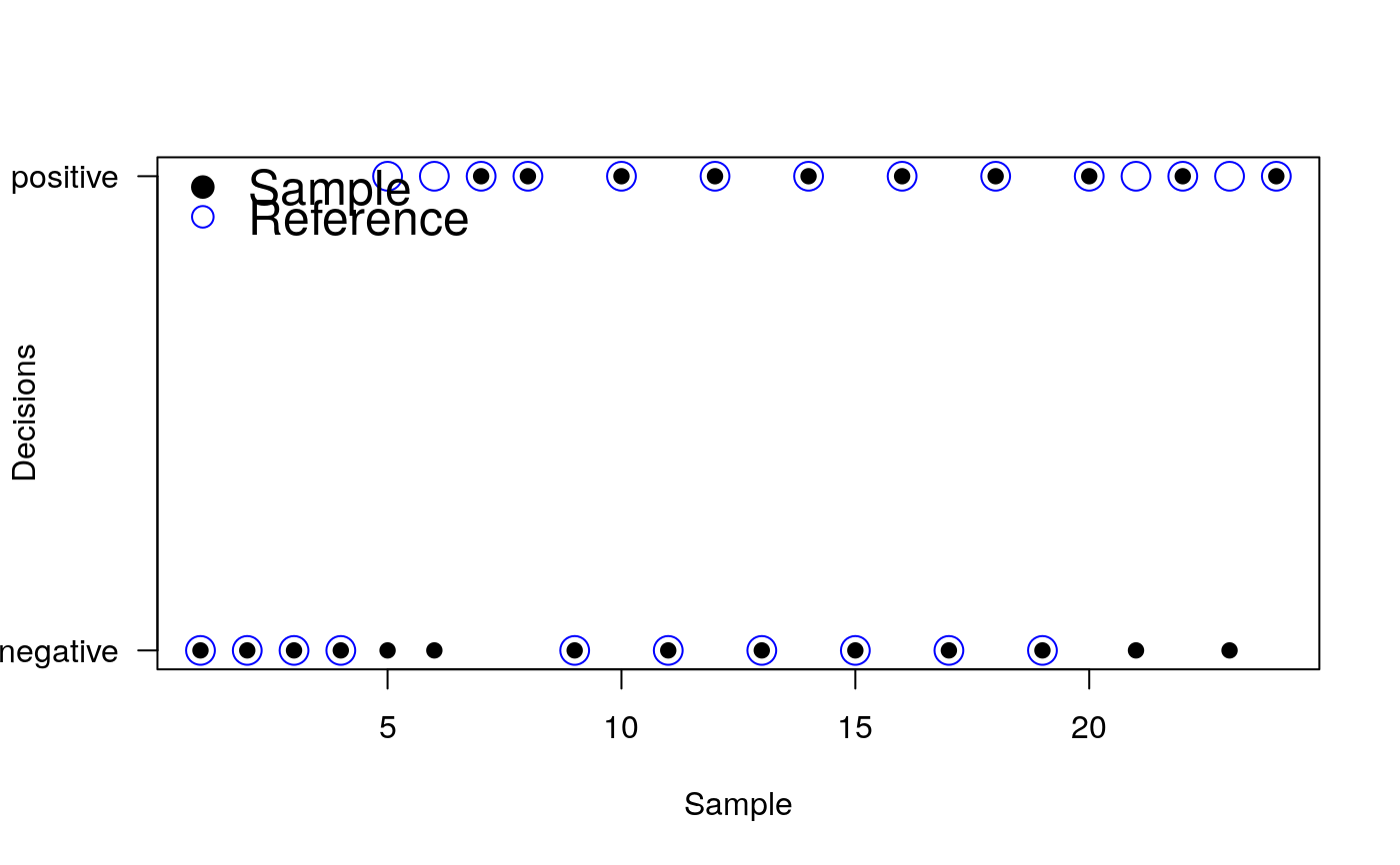
Examples
# Produce some arbitrary binary decisions data # test_data is the new test or method that should be analyzed # reference_data is the reference data set that should be analyzed test_data <- c(0,0,0,0,0,0,1,1,0,1,0,1,0,1,0,1,0,1,0,1,0,1,0,1) reference_data <- c(0,0,0,0,1,1,1,1,0,1,0,1,0,1,0,1,0,1,0,1,1,1,1,1) # Plot the data of the decisions plot(1:length(test_data), test_data, xlab="Sample", ylab="Decisions", yaxt="n", pch=19)legend("topleft", c("Sample", "Reference"), pch=c(19,1), cex=c(1.5,1.5), bty="n", col=c("black","blue"))# Do the statistical analysis with the performeR function performeR(sample=test_data, reference=reference_data)#> TPR SPC PPV NPV FPR FNR FDR ACC F1 MCC #> 1 0.7142857 1 1 0.7142857 0 0.2857143 0 0.8333333 0.8333333 0.7142857 #> LRp kappa TP TN FP FN counts #> 1 Inf 0.6756757 10 10 0 4 24