winklR: A function to calculate the angle based on the first and the second derivative of an amplification curve data from a quantitative PCR experiment.

winklR is a function to calculate the in the trajectory of the first and the second derivatives maxima and minima of an amplification curve data from a quantitative PCR experiment. For the determination of the angle (central angle), the origin is the maximum of the first derivative. On this basis, the vectors to the minimum and maximum of the second figure are determined. The vectors result from the relation of the maximum of the first derivative to the minimum of the second derivative and from the maximum of the first derivative to the maximum of the second derivative. In a simple trigonometric approach, the scalar product of the two vectors is formed first. Then the absolute values are calculated and multiplied by each other. Finally, the value is converted into an angle with the cosine. The assumption is that flat (negative amplification curves) have a large angle and sigmoid (positive amplification curves) have a smaller angle. Another assumption is that this angle is independent of the rotation of the amplification curve. This means that systematic off-sets, such as those caused by incorrect background correction, are of no consequence. The cycles to be analyzed is defined by the user. The output contains the angle.

winklR(x, y, normalize = FALSE, preprocess = TRUE)

Arguments

x	is the cycle numbers (x-axis). By default the first ten cycles are removed.
y	is the cycle dependent fluorescence amplitude (y-axis).
normalize	is a logical parameter, which indicates if the amplification curve data should be normalized to the 99 percent percentile of the amplification curve.
preprocess	is a logical parameter, which indicates if the amplification curve data should be smoothed (moving average filter, useful for noisy, jagged data).

See also

acos diffQ2

Examples

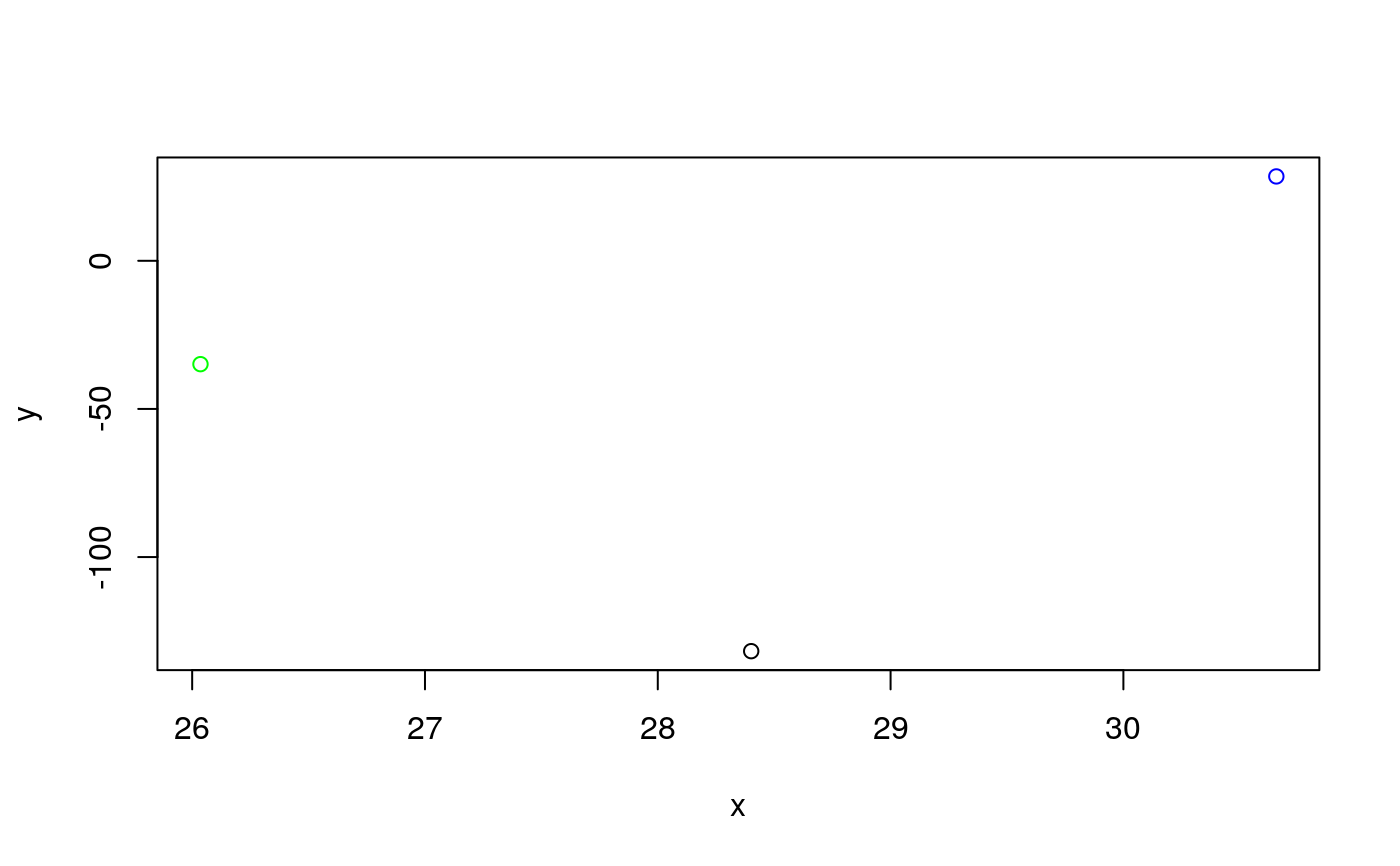
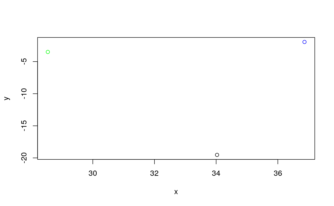
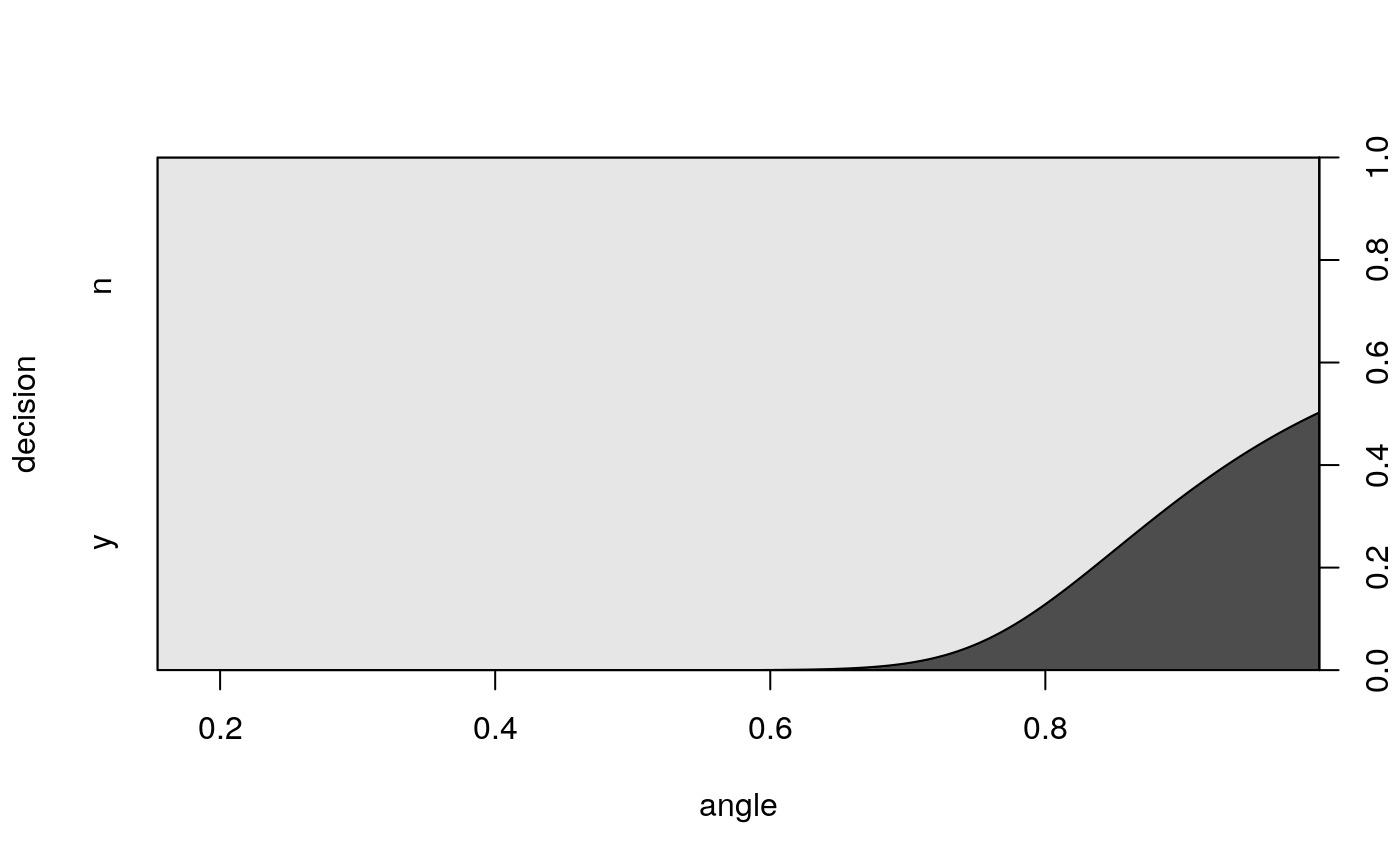
# Calculate the angles for amplification curve data from the RAS002 data set
data(RAS002)

# Plot the data
plot(RAS002[, 1],
  y = RAS002[, 2], xlab = "Cycle", ylab = "RFU",
  main = "RAS002 data set", lty = 1, type = "l"
)
res <- winklR(x = RAS002[, 1], y = RAS002[, 2])
res
#> $angle
#> [1] 0.9992592
#> 
#> $origin
#>               x         y
#> origin 28.40128 -131.7579
#> 
#> $p1
#>           x         y
#> p1 26.03566 -34.89072
#> 
#> $p2
#>           x        y
#> p2 30.65694 28.46814
#> 
plot(rbind(res$origin, res$p1, res$p2), col = c("black", "green", "blue"))

plot(RAS002[, 1],
  y = RAS002[, 7], xlab = "Cycle", ylab = "RFU",
  main = "RAS002 data set", lty = 1, type = "l"
)
res <- winklR(x = RAS002[, 1], y = RAS002[, 7])
res
#> $angle
#> [1] 0.8825469
#> 
#> $origin
#>               x         y
#> origin 34.02938 -19.53181
#> 
#> $p1
#>           x         y
#> p1 28.54223 -3.497543
#> 
#> $p2
#>           x         y
#> p2 36.86468 -1.942902
#> 
plot(rbind(res$origin, res$p1, res$p2), col = c("black", "green", "blue"))

res_angles <- unlist(lapply(2:21, function(i) {
  winklR(RAS002[, 1], RAS002[, i])$angle
}))
cdplot(RAS002_decisions[1L:20] ~ res_angles, xlab = "angle", ylab = "decision")